How to implement the Newton-Method

Hi, after a long time I thought I would do something on Newton's method, since it is quite an important topic in mathematics.

Well, we don't do mathematics here in the sense, rather we look at how the method works and how you can implement this programming.

What is the newton Newton-Method?

First, we need to know what the Newton method actually is. Newton's method is an unstable method, with which we can quickly find zeros of a known function. It is much faster than the bisection method, with which we can also find zeros.

Unstable?

Why unstable? Quite simply, there are situations where one does not come with this procedure on a zero, since for one e.g. only a saddle point was reached or at a bad place was started.

If the function is known, you can use the first derivative to get closer and closer to the zero. More precisely, we have chosen an X-value and subtract that from the quotient. The quotient is a combination of the function and the derivative of the function. Both get the chosen x-value as well. The general formula is:

$$x_{n+1} = x_{n} - \frac{f(x_{n})}{f'(x_{n})}$$

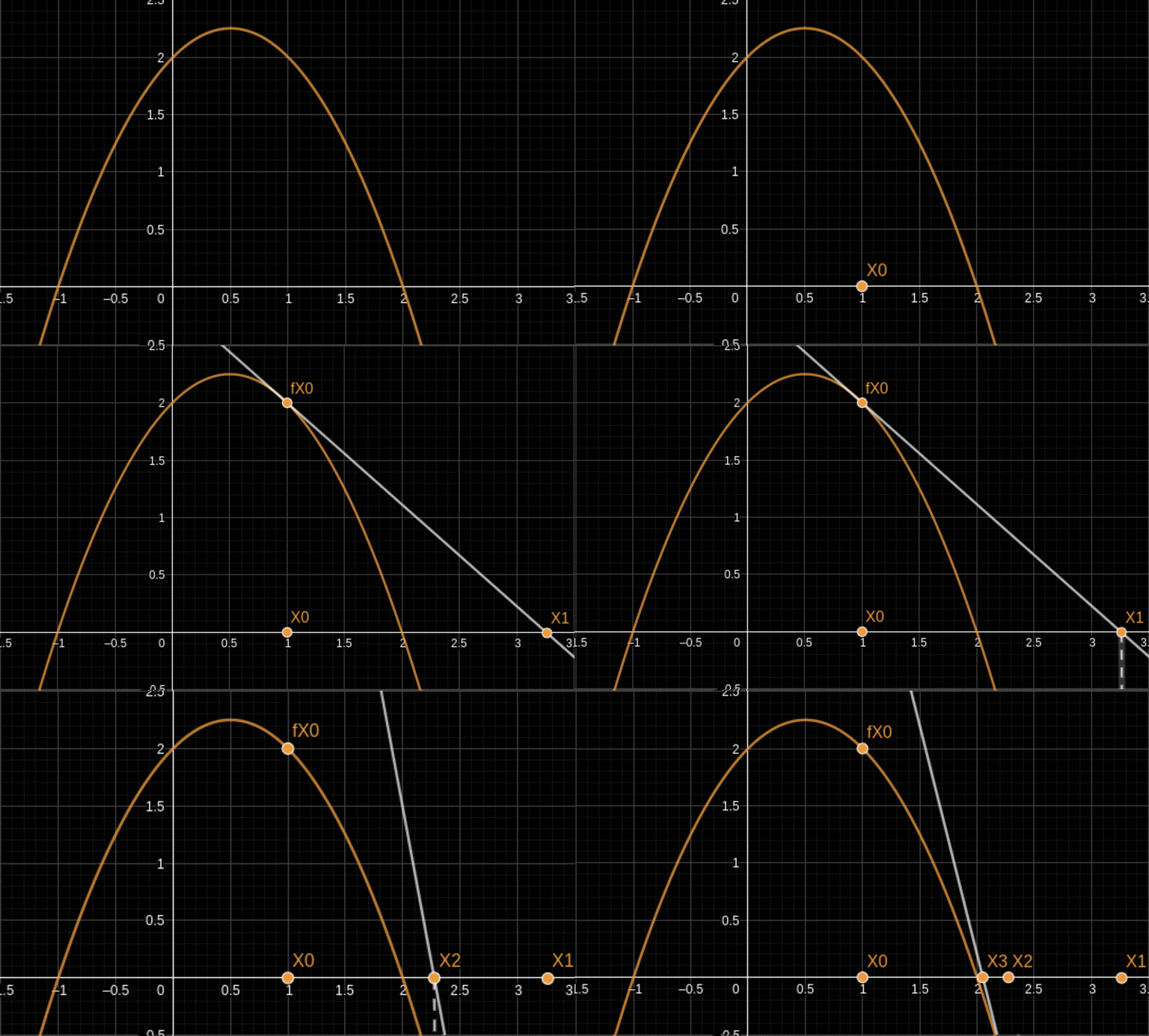
Ok, we see that the formula is quite simple, but the question is, what actually happens? We know that Newton's method quickly approaches a zero point with the help of tangent equations. Assuming we have a function $f(x)$, which is known to us, we can see from the animation what exactly happens there.

In the picture above, you can see well how exactly the Newton method works. First a point $X_{0}$ is chosen. Here it is important that the start value of the Newton iteration is chosen in such a way that this is between 2 extreme points or the derivative value, i.e. the gradient at the point $X_{0}$, is greater or smaller than 0. Otherwise, the method can find no zeros or one gets everything other than the zeros out.

The function value at the point $X_{0}$ is the point of contact of the tangent. The slope is followed further and further in the X-direction as shown in the animation above. At the point where the tangent intersects the X-axis, is the next X-value, which is inserted into the function. The whole thing is then repeated until the zero point is approached very precisely or lands on it. Here you get a convergence to the zero.

If one has chosen an unfavorable $X_{0}$, it diverges or one moves further and further away from the zero and one must then choose a new $X_{0}$. But you do not only have to move away from the zero, there are cases where by a bad $X_{0}$, the method jumps back and forth between 2 values, which is also a form of divergence.

In order to form the derivative, which the computer cannot do, one can simply enter the derivative of the function in such a way or one applies as it is usual in most cases, a numerical procedure e.g. with the h-formula. This formula does nothing else than, with a parameter $h$, which one lets run against 0, to form our derivative. The h-formula then looks like this:

$$\lim_{h \to 0}: \frac{f(x_{0} + h)-f(x_{0})}{h} = f'(x_{0})$$

Implement the Newton-Method

Ok, now we know enough and can begin with the tinkering. The whole, we convert simply times in C++. First of all, we should think about whether we simply build in the derivative or approximate it using the h-formula. I will do this by means of the h-formula. First we create the newton.h, in which the method and the h-formula is implemented. To be able to pass the functions later, a function pointer is created by typedef. The header file should look like this.

#include <math.h>
#ifndef NEWTON_H
#define NEWTON_H

typedef double (*function)(double x);
double newton(double xn, double (*f)(double x));
double formular_h(double (*f)(double x), double x);

#endif //NEWTON_H

What is missing now is the implementation associated with the function prototypes, which is done in the newton.cpp.

#include "newton.h"
double newton(double xn, double (*f)(double x))
{
    return xn - f(xn)/formular_h(f, xn);
}

double formular_h(double (*f)(double x), double x)
{
    return (f(x + H) - f(x))/H;
}

You can see now that it is quite easy to implement, since the procedure is now kept quite simple in the state. What is only missing is the parameter H, which should be as small as possible. As value for the parameter H, $10^{-8}$ is chosen, because it is already very small or close to 0. The whole, can then be defined by means of a #define H 10-E8. With this we have already implemented the procedure itself and can now just let it run. To do this, we first create a function $f(x) = -x^{2} + x + 2$, which we have already seen in the animation above.

The whole thing, we can write in the main.cpp and pass this later in the procedure, as a pointer. The implemented function should then look like below.

#include <iostream>
#include "newton.h"

double f(double x)
{
    return -1* pow(x, 2) + x + 2;
}

In order to make the procedure executable, we should first select an $X_{0}$, which can provide us with a guaranteed zero. For this $X_{0} = 1$ would be a suitable value. We let the procedure run for 10 steps, so that we can see the convergence to 2. To assign the function $f(x)$ to a function pointer, we should first set a pointer, which we call pFunc. This pointer is simply assigned the name of the function, in this case f.

The main function should then look something like this:

int main()
{
    function pFunc = f;
    double xn = 1;double xn_1 = 0;
    for(int i = 0; i < 10; i++)
    {
        std::cout << "Newton-iteration " << i << "..." << std::endl;
        xn_1 = newton(xn, f);
        std::cout << "XN+1 = " << xn_1 << std::endl;
        xn = xn_1;
    }
 
    return 0;
}

Here, the value $X_{n+1}$ is calculated and output per iterarion step. So we can see if we are approaching the zero or not. The $X_{n}$ is the previous value, which is replaced by $X_{n+1}$ after the output. Ok, let's compile this and let it run.

And this is how the whole thing looks:

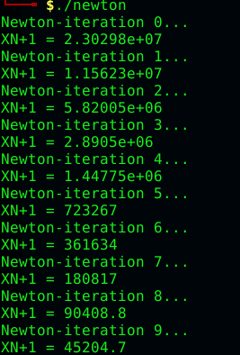
We see that Newton's method works and we end up at the 4th iteration step exactly at the zero point 2, which was again outlined in red. If we had taken the value -0.5 for $X_{0}$, we would have landed at the zero -1. With all values except the 0.5, we would have landed here with one of the two zeros. Below I have added a picture to show what happens if you choose an unfavorable value for $X_{0}$.

Here we see that the method diverges for an $X_{0} = 0.5$. This is due to the fact that we have the vertex of the parabola at the point $X = 0.5$, and here the slope is 0.

The code can also be found on Github.

I hope you enjoyed it and see you next time 😄