What are Graphs?

Graphs are data structures that form a kind of network. These come from graph theory and are nothing more than a set of nodes and edges, which are all somehow connected to each other. With graphs many everyday problems can be modeled e.g. city map, navigation systems etc...

Graphs are also used in network technology. Here the network is represented as a graph, so that routers form the nodes, and routed accordingly.

Here I don't want to go into how graphs are programmed but rather scratch around on the surface a bit.

Definition of a Graph

Let $G = (K, E)$ where $G$ is the graph and $K$ is the set of all nodes and $E$ is the set of all edges. With this information, one can build graphs.

A small example:
$G = (K, E)$
$K = \{A, B, C\}$
$E = \{(A, B), (A, C), (C, B)\}$

Then our graph would look like this when we build everything together.

Types of Graphs

There are basically 2 types of graphs, directed and undirected graphs.

A directed graph looks like this:

An undirected graph looks like this:

Note that not every directed graph can be converted to an undirected graph. The reason is that with an undirected graph, we can go from $A$ to $B$, or from $B$ to $A$.

Let's code some graphs

Ok, what can we do with it now? Let's assume we now want to know which paths there are to get from $A$ to $F$ for these graphs.

Naively, it would be a good idea to start from node $A$ and simply walk along all the paths. And that's exactly what we'll do now.

The paths are:

$A \rightarrow D \rightarrow F$
$A \rightarrow D \rightarrow E \rightarrow F$
$A \rightarrow D \rightarrow B \rightarrow C \rightarrow E \rightarrow F$
$A \rightarrow B \rightarrow C \rightarrow E \rightarrow F$
$A \rightarrow B \rightarrow C \rightarrow D \rightarrow F$
$A \rightarrow B \rightarrow C \rightarrow D \rightarrow E \rightarrow F$

The same can be done to any node in the graph.

A small implementation in Prolog shows how to implement such a graph.

%edge(X, Y) X goes to Y
edge(a, b).
edge(a, d).
edge(b, c).
edge(c, d).
edge(c, e).
edge(d, e).
edge(d, f).
edge(e, f).
%edge(f, a).


path(X, X).
path(X, Y) :- edge(X, U), path(U, Y).

route(X, X, list(X, nil)).
route(X, Y, list(X, Xs)) :- edge(X, N), route(N, Y, Xs).

Note that I have commented out the edge $F \rightarrow A$ because it comes to loops. Here a cycle recognition would have to purely, which would make however the code very unclear. Well no matter if we run the times we will see what happens.

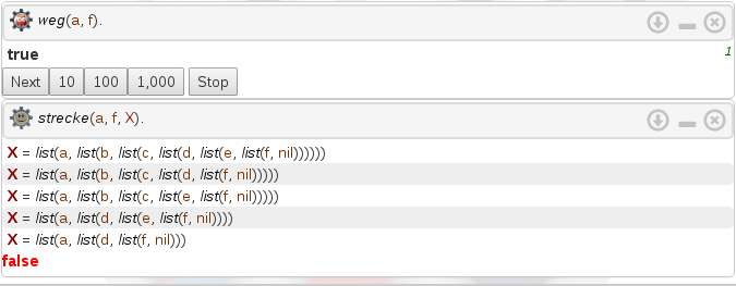
The language used in the following image is german

In the output we see that when we ask Prolog if there is a path from node $A$ to node $F$, it returns true. In the next query we ask which paths exist and we get solutions thrown out. Prolog did not find all paths, but this is due to the depth-first search.

Adjacency matrix

A graph can also be represented in the form of an adjacency list or adjacency matrix.

For the adjacency matrix we do the following, we create a row for each node. Then create exactly as many columns of the same label.

This then looks like this:

	A	B	C	D	E	F
A
B
C
D
E
F

Now that we have created everything, we can start filling the matrix. We go through the matrix column by column. At node $A$ we look where we can get everywhere. From node $A$ we come out at $B$ and $D$. We keep doing this until the matrix is full.

	A	B	C	D	E	F
A	0	1	0	1	0	0
B	0	0	1	0	0	0
C	0	0	0	1	1	0
D	0	1	0	0	1	1
E	0	0	0	0	0	1
F	1	0	0	0	0	0

What exactly does the matrix bring us?
We can represent this matrix as a two-dimensional array, and thus store graphs in files and read them out again.

Adjacency list

Another possibility is, as already mentioned, the adjacency list. This has a similar structure but a bit more memory efficient than the matrix. Here we have a one-dimensional array which contains lists. Also here we look where we come out at the single nodes.

This looks like this:

$[A] \rightarrow B \rightarrow D$
$[B] \rightarrow C$
$[C] \rightarrow D \rightarrow E$
$[D] \rightarrow B \rightarrow E \rightarrow F$
$[E] \rightarrow F$
$[F] \rightarrow A$

Great, now we have learned a few things about graphs, but what about graphs with weights on the edges?

Weights

First of all, what is a weight?
A weight is a real number, which represents e.g. the distance. Suppose we have a map and want to go from Aachen to Berlin. Here we would have different cities that are on the way and connected to Aachen and Berlin. Each route has a certain length. Each city is connected to another city by a highway. We want to know the shortest way to get to Berlin. There the weights (distance further) help us.

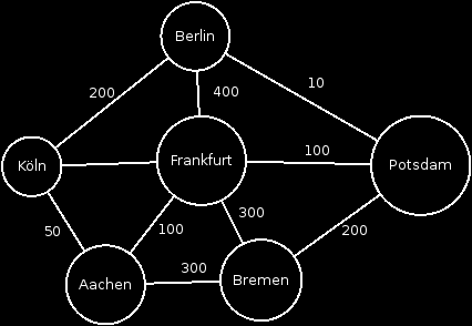
A graph with weighted edges looks like this:

The edges have all got numbers as mentioned these are the weights. The weights here are the kilometers we need to get from Aachen to Berlin. The other cities are possible intermediate stops. The kilometer numbers are only exemplary.

Here we can also go naively to the thing, in which we visit from Aachen all nodes and count the kilometers.

Aachen $\rightarrow$ Bremen $\rightarrow$ Potsdam $\rightarrow$ Berlin = 510Km
Aachen $\rightarrow$ Frankfurt $\rightarrow$ Berlin = 500Km
Aachen $\rightarrow$ Köln $\rightarrow$ Berlin = 250Km
Aachen $\rightarrow$ Frankfurt $\rightarrow$ Potsdam $\rightarrow$ Berlin = 210Km
...

I think you can see where this leads to. To algorithms, which look for us the shortest ways out e.g. Prim, Kruskal, Dijkstra etc...

I will go into this in the next post.

I hope I could provide a little insight into graphs 😄